How an LLM works: from your question to the first word

You type: "Summarise this contract in three points". You press Enter. Half a second of silence. Then the words arrive, in a steady stream.

During that silence, your sentence was cut into tokens, small pieces of words, then turned into numbers. Those numbers went through dozens of layers of a neural network, the transformer. All of that to produce… a single token.

And that token is not decided in advance. The model computes a probability for every possible continuation, then draws one at random among the most likely. It is non-deterministic: the same question can give two different answers.

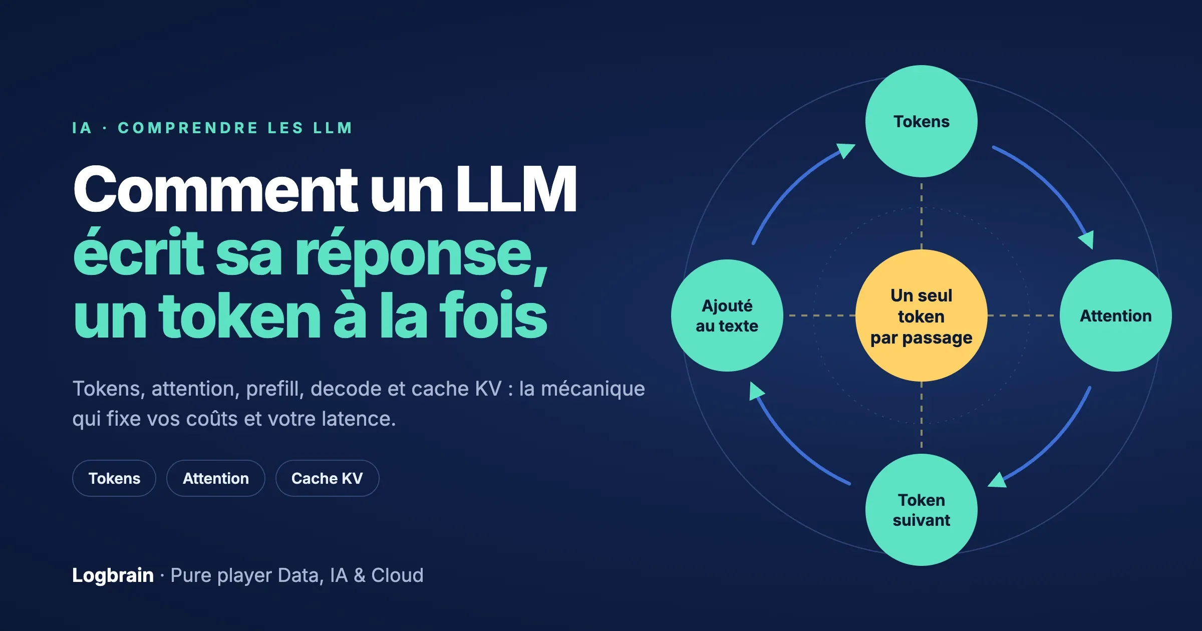
Then it starts again. The new token is appended to the text, and the model predicts the next one, token after token, until the final full stop. This is called autoregressive generation.

This mechanism explains what you see in your company:

• a price counted in tokens;
• a wait before the first word;
• answers that change from one try to the next;
• a prompt order that can change the bill.

Let's follow that sentence, step by step.

The principle: guessing what comes next

An LLM (Large Language Model) does only one thing: given a text, it guesses the next piece of text. No ready-made answers, no encyclopedia lookup.

It is your phone's autocomplete, at a colossal scale. To guess the continuation of any text well, the model had to learn grammar, facts, reasoning and code.

In practice, a model is two things:

• an architecture, the calculation formula. Almost every LLM uses the same one: the transformer;
• weights (or parameters), billions of numbers tuned during training. All of the model's "knowledge" lives there.

From one model to the next, the architecture changes little. The difference comes mostly from the weights, and therefore from the training data.

At its core, an LLM is a giant mathematical function. It takes a sequence of numbers as input and produces a number as output.

Inside, there is an enormous graph of operations: billions of carefully arranged calculations that turn the input numbers into that output number.

This graph can be roughly split into four parts.

The text goes through these four parts to produce a single token. That token is appended to the text, and the cycle starts again, until a special token that means "end". Let's take each part in order.

Step 1: tokens

Before it can do anything, the model has to turn your text into something it can handle: numbers. That is the job of the tokenizer.

It cuts the prompt into small pieces and gives each piece a number: its token. Here is our sentence run through OpenAI's tokenizer, the one used by GPT-4o and GPT-5:

The sentence becomes the list ["Summ", "ar", "ise", " this", " contract", " in", " three", " points"], then the numbers [64614, 277, 1096, 495, 6698, 306, 3407, 5571]. For the model, your question is nothing more than that.

Three details matter:

• the same sentence always gives the same tokens;
• the space is part of the token: "␣contract" is a single piece;
• capitals matter: " contract" in the middle of a sentence is token 6698, "Contract" at the start is 14221, and "contract" with no space before it is 26186. A capital tells you something about the word: "Will" is probably a name, "will" a verb.

Tokens are the basic unit, both in and out. Let's ask the model a question to see it in action. Press ↑ when you are ready:

Numbers go in, the computation happens, one number comes out. The tokenizer turns it back into text, and it appears on screen. That is why the answer arrives token by token, in small pieces.

Notice also that every token produced is appended to the input before the next round. The model needs everything: without the question, it would forget what it was asked; without the start of its answer, it would keep producing the first word.

There are also special tokens. One of them means "end of answer": at OpenAI, it is number 199999, the one that ends the answer above. When the model produces it, it stops. Others mark the start and end of each message: that is how a chat model knows where your question ends and its answer begins.

What this means in practice:

• you pay in tokens, the ones you send and the ones the model writes;
• every provider has its own tokenizer: the same text does not cost the same everywhere. You can compare them on tiktokenizer;
• other languages and code cost more than English, because they are split more finely;
• counting the letters in a word is hard for a model that only sees pieces.

import tiktoken

tok = tiktoken.get_encoding("o200k_base")
ids = tok.encode("Summarise this contract in three points")
print([tok.decode([i]) for i in ids])  # the pieces

Step 2: embeddings

The tokenizer left us with numbers. Problem: those numbers mean nothing. "contract" is number 6698, but 6699 has nothing to do with it. You cannot compute anything meaningful with a label.

So the model replaces each number with an embedding: a long list of numbers, called a vector, that describes the meaning of the token.

A huge lookup table

The model contains a giant table with one row per token in the vocabulary. Token 6698 fetches row 6698. No calculation: a simple lookup.

Each row holds thousands of numbers: 7,168 for DeepSeek-V3, for example. With a vocabulary of 129,000 tokens, its table alone weighs nearly a billion parameters.

Nobody writes these numbers. At the start they are random. Training adjusts them, little by little, until they help guess the next token well.

Meaning becomes geometry

A vector is a point in a space with thousands of dimensions. And training arranges those points in a remarkable way: words with similar meanings end up close to each other.

Even directions carry meaning. Going from "France" to "Paris" looks like going from "Italy" to "Rome". In the first embedding models (word2vec, 2013), the calculation "king − man + woman" landed very close to "queen". Nobody programmed that: it emerged from training.

No dimension is called "gender" or "country". Meaning is spread across all of them at once, in a way researchers are only starting to decode.

How many dimensions?

The diagram shows only two, so the words can be drawn on a page. A real model uses thousands. Why so many?

Because a word has many facets. With two dimensions, "bank" has to choose: close to rivers or close to money. With thousands, it can be close to both at once, along different axes. Each extra dimension is room for one more nuance.

This number is called the model dimension, its "width". Every token keeps a vector of that size from end to end, through every layer. A few recent models:

• gpt-oss-120b (OpenAI, 2025): 2,880;
• Qwen3 8B (Alibaba, 2025): 4,096;
• Llama 4 Maverick (Meta, 2025): 5,120;
• DeepSeek-V3 and Kimi K2: 7,168.

Closed models (GPT-5, Claude, Gemini) do not publish this figure.

Notice that width no longer follows size: gpt-oss-120b has 120 billion parameters, with vectors of only 2,880 numbers. Recent models grow mostly by adding experts (the Mixture of Experts architecture), not by widening the vectors.

More dimensions means more nuance, but also more computation and memory for every token processed.

One vector per word, whatever the context

At this stage, each token has a single vector, always the same. "bank" has the same embedding in "the river bank" and in "the bank raised its rates": a point somewhere between the river and the money.

The following layers will pull it one way or the other by looking at the surrounding words. That is step 3. But first, one essential piece of information is missing.

Word order: position embeddings

The embedding of "John" is the same wherever it appears in the sentence. Without anything else, "John eats the apple" and "The apple eats John" give exactly the same vectors: to the transformer, they are the same thing.

So it has to be given the position of each token. Three methods followed one another:

• the fixed formula, called sinusoidal (the original transformer, 2017): the position is computed with sines and cosines, then added to the embedding. Nothing to learn;
• the learned position (GPT-2, BERT): a table with one vector per position, tuned during training like everything else. More flexible, but limited: GPT-2 learned 1,024 positions, BERT 512. Beyond that, there is simply no vector for the next position;
• RoPE (Rotary Position Embedding), today's standard (Llama, Mistral, Qwen…): a fixed formula, but a smarter one. Instead of adding the position to the embedding, it rotates the vectors by an angle that depends on the position, at the moment words are compared in attention.

With RoPE, what matters is the distance between two words, not their absolute place. "John" two words before "eats" gives the same relationship whether the sentence is at the start of the text or at token 50,000. It is one of the keys that made it possible, with a few adjustments, to extend context windows to hundreds of thousands of tokens.

Step 3: the transformer

This is the heart of the model, and where almost all the computation happens. The transformer is a stack of identical blocks called layers: 36 for Qwen3 8B or gpt-oss-120b, 61 for DeepSeek-V3.

Each layer has two stages:

1. attention: each word looks at the others and draws information from them;
2. feedforward: each word, on its own, "thinks about" what it has just learned.

A layer does not replace a word's vector: it adds a correction to it. Layer after layer, the vector of "bank" drifts towards the river or towards money, depending on the sentence. This is called the residual stream: a current that flows through the whole stack and gets richer at every stage.

Attention: every word looks at the others

Take our answer in progress: "The contract lasts". To guess what comes next, "lasts" needs to know what lasts. So it looks mostly at "contract".

How does a word know where to look? Each layer has learned three matrices. Multiplying each word's vector by them gives three new vectors:

• a query (Q): what I am looking for;
• a key (K): what I offer;
• a value (V): what I pass on if I am chosen.

Like in a meeting: everyone has a question in mind, reads the others' badges, and listens mostly to the people who can help.

The calculation, step by step

Let's do it by hand, on four tokens. To keep it readable, each vector here has only two numbers. In reality, it has about a hundred per head.

1. Compare. Each word's query is multiplied by every word's key: this is the dot product. For "lasts" and "contract": (1, 1) · (1, 2) = 1×1 + 1×2 = 3. The more two vectors point in the same direction, the higher the score.
2. Mask. Above the diagonal is the future: "lasts" cannot look at "three", which has not been written yet. We put −∞ there.
3. Normalise. The softmax turns each row into weights that add up to 100%: take the exponential of each score, then divide by the total. For "lasts": e¹ = 2.7, e³ = 20.1 and e² = 7.4, that is 9%, 67% and 24%. The exponential of −∞ is 0: the future weighs exactly 0%.
4. Mix. The new vector of "lasts" is the sum of the values, weighted by those weights: 9% of "The", 67% of "contract", 24% of itself. It now mostly carries the information of "contract".

Two differences with reality. The scores are also divided by the square root of the vector size, to keep them from growing too large. And the grid is not 4 × 4: with 100,000 tokens of context, it has 10 billion cells, for every head of every layer. That is why long contexts are so expensive.

All of these calculations are matrix multiplications. That is exactly what GPUs do massively, and in parallel.

import numpy as np

def attention(Q, K, V):
    scores = Q @ K.T / np.sqrt(K.shape[-1])           # 1. compare
    future = np.triu(np.ones_like(scores), k=1) == 1
    scores[future] = -np.inf                          # mask: no future
    weights = np.exp(scores)
    weights /= weights.sum(-1, keepdims=True)         # 2. softmax
    return weights @ V                                # 3. mix

Three kinds of attention

Depending on who is allowed to look at whom, there are three kinds of attention.

• Self-attention: each word looks at every word of the same text, before and after. Ideal for understanding a whole sentence at once.
• Masked self-attention (or causal): each word only looks at the previous words. A mask hides the future. It is essential for generating: when the model writes the third word, the fourth does not exist yet.
• Cross-attention: the queries come from one text, the keys and values from another. The text being written questions a text already read.

The mask brings two bonuses. During training, it lets the model learn every position of a sentence in a single pass. And during inference, it guarantees that a word's computation never changes once done: that is what will make the KV cache possible.

Encoder, decoder: three families of models

The original transformer (Google, 2017) was built for translation. It had two parts:

• an encoder, which reads the source sentence with self-attention;
• a decoder, which writes the translation with masked self-attention, and consults the encoder through cross-attention.

Since then, each half has gone its own way:

• encoder-only (BERT, ModernBERT): understanding, classifying, producing embeddings for search. It does not generate text;
• encoder-decoder (T5, Whisper): turning one text into another, or speech into text;
• decoder-only (GPT, Claude, Llama, Qwen, DeepSeek): generating, token after token.

Decoder-only won for LLMs. It is simpler, a single stack, and it reduces every task to one: continuing a text. Translating, summarising or answering become special cases. And it trains on any text, without question-answer pairs.

Several heads in parallel

A single attention can only follow one type of relationship at a time. So each layer runs dozens of them in parallel, the heads: 64 for gpt-oss-120b, 128 for DeepSeek-V3.

Nobody assigns them a role. But when researchers observe them, they find heads that link a verb to its subject, a pronoun to its noun, or an opening bracket to its closing one.

Recent models make several heads share the same keys and values: this is GQA (Grouped-Query Attention). Qwen3 8B has 32 query heads for only 8 key and value heads. Quality barely drops, and the KV cache memory is divided by four.

Feedforward: where knowledge is stored

After attention, each vector goes alone through the feedforward: a small network that enlarges it (three to four times), transforms it, then brings it back to its size.

It looks like nothing, but it holds about two thirds of the parameters. Researchers see it as a kind of memory: it is where the model stores much of what it knows, such as "Paris is in France".

It is also where experts come in. In a Mixture of Experts model, the feedforward is split into many small networks, and a router activates only a few of them for each token. DeepSeek-V3 has 671 billion parameters but uses only 37 billion per token. The model knows a lot, but computes little.

At the top of the stack

After the last layer, the vector of the last token has absorbed everything: the question, the context, the start of the answer. All that remains is to turn it into a word. That is step 4.

Step 4: the output, choosing the next token

We leave the stack with a single useful vector: the one of the last token, which has absorbed everything. In DeepSeek-V3, it is a list of 7,168 numbers. Now we need a word out of it.

From vector to scores: logits

The model has a second table, the mirror of the embedding table: one row per token in the vocabulary. Some models even reuse the same one.

It compares the vector with each of these rows, using a move we already know: the dot product. The more the vector resembles the row for "three", the higher the score for "three".

The result is a score for each of the 200,000 tokens in the vocabulary. These raw scores are called logits. After "The contract lasts", for example:

• "three": 3;
• "two": 2.2;
• "five": 1.6;
• "one": 1.1;
• "pizza": −1.5.

From scores to probabilities: softmax, again

To turn scores into probabilities, it is the same softmax as in attention: the exponential of each score, divided by the total.

The exponentials are 20.1 for "three", 9.0 for "two", 5.0 for "five", 3.0 for "one" and 0.2 for "pizza". Out of a total of 37.3, that gives 54% for "three", 24% for "two", 13% for "five", 8% for "one" and 0.6% for "pizza".

The model does not choose "three". It draws at random according to these probabilities: about one time in two, it will write something else.

Temperature: sharpening or flattening

Before the softmax, all the logits are divided by a number: the temperature.

• Temperature 1: nothing changes. "three" has a 54% chance.
• Temperature 0.5: the gaps double, the favourite crushes the others. "three" rises to 78%.
• Temperature 1.5: the gaps shrink, the outsiders come back. "three" drops to 43%, and "pizza" goes from 0.6% to 2%.
• Temperature 0: no more randomness, the top token always wins. This is greedy mode.

Cutting the tail: top-k, top-p, min-p

Our example has only five candidates. The real one has 200,000, including thousands of absurd ones at 0.001%. One by one, they are negligible. Together, they end up coming out, especially at high temperature.

So this tail is cut before the draw:

• top-k: keep the k best, for example the top 40;
• top-p: keep the best until reaching p% of cumulative probability. With top-p at 90%, "three", "two" and "five" are enough (91%): "one" and "pizza" are removed;
• min-p: keep those that weigh at least a fraction of the favourite, for example 10%. The cut adapts by itself: tight when the model is confident, wide when it hesitates.

The remaining probabilities are scaled back to 100%, then the draw happens.

Why two different answers

This draw is what makes the model non-deterministic, as announced at the start. Same question, same model: a different draw on the first token, and everything after it diverges.

Even at temperature 0, two calls can differ slightly. On servers, your request is computed in a batch with other users' requests, and the order of additions changes from one time to the next. Rounding shifts by a hair, and sometimes that is enough to change the favourite.

Some reasoning models do not even let you set the temperature: the provider fixes it.

Enforcing a format: structured output

When you ask for JSON, the engine can do better than hope. Before each draw, it sets to −∞ the logits of every token that would break the format: free text where a brace is needed, a number where a string is needed.

It is exactly the mask trick from attention. The exponential of −∞ is 0: those tokens can no longer come out. The JSON is valid by construction.

And again

The drawn token is appended to the text, and everything goes back into the model: it is the loop we saw with the chat window in step 1. It stops at the end token, or when the length limit set by the call (max_tokens) is reached.

Prefill and decode: the two phases of generation

We now know what happens inside the model. Let's look at the same thing from the machine's side, because that is where your bill and your waiting time are decided.

A reminder first: during inference, the model learns nothing anymore, its weights are frozen. Training happens once. Inference runs billions of times, for every question from every user. That is where the cost lives.

And inference is not one operation but two, which behave in opposite ways.

Phase 1: prefill, the whole prompt at once

You send a 2,000-token prompt. The model knows all of them from the start. So it can process them in parallel: at each layer, every token computes its query, key and value, and the attention grid from step 3 is computed in full, in a single block.

These are huge matrix multiplications. The GPU's compute units run flat out: prefill is said to be compute-bound.

Prefill produces two things:

1. the first token of the answer;
2. the KV cache: at each layer, the keys and values of the 2,000 tokens, stored in GPU memory.

The queries are not kept. A query is a token's question at the moment it is processed. Keys and values are the past, which every following token will consult. They stay.

Prefill is the silence at the start: the time to first token, or TTFT.

Phase 2: decode, one token at a time

The first token goes back into the model. But this time, it is alone.

It computes its query, key and value. Its key and value are added to the cache. Its query questions every key in the cache: the 2,000 from the prompt, plus those of every token already written. In the attention grid, only one row is computed now, the last one.

Out comes a new token, which goes back in turn. This is the autoregressive loop: each token depends on the previous one, so it cannot be parallelised.

And here is the problem. For that single token, the GPU has to reread all the model's weights and the whole cache from memory. Very little computation, an enormous amount of reading. Decode is memory-bound, or more precisely limited by memory bandwidth.

Let's do the maths. An 8-billion-parameter model weighs 16 GB in 16-bit. An H100 GPU reads its memory at about 3,350 GB per second. For each token, those 16 GB must be reread: 200 tokens per second at best, even though the compute units are almost idle.

Hence the servers' trick: batching. Since the weights have to be reread anyway, the same read is used to move 32 or 64 users' answers forward by one token at once. One read, dozens of tokens.

Decode is the stream: the time per output token, or TPOT.

Two phases, two bottlenecks

• Prefill processes the whole prompt in parallel. It is limited by compute, and it sets the wait before the first word. It grows with the size of the prompt.
• Decode processes one token at a time. It is limited by memory reads, and it sets the speed of the stream. It grows with the length of the answer.

Same model, same request, but two opposite hardware profiles. That is why inference optimisation is a craft of its own, and why large deployments go as far as running the two phases on different machines.

The four metrics to know

• TTFT: the wait before the first token. Mostly prefill, but also queuing and the network.
• TPOT: the time between two tokens once the stream has started. Mostly decode.
• Throughput: the total number of tokens produced per second, across all users.
• End-to-end latency: from sending to the end of the answer. Roughly TTFT + number of tokens × TPOT. An answer of 500 tokens at 30 ms per token, after a 0.5 s wait: 15.5 seconds.

The first two are what the user feels. Throughput and cost per token are what your finance team feels. And they pull in opposite directions: putting more users in the same batch increases throughput but slows each of them down. Optimising inference means picking the right point on that curve.

What it means for you

• Output tokens cost more than input tokens, often 4 to 8 times more: they go through decode one by one;
• a long document delays the first word, but barely slows down the rest;
• a long answer costs time and money: asking for "three points" is an optimisation;
• streaming is essential: showing tokens as they come hides the wait.

The KV cache: never recompute the past

The KV cache is born during prefill. Let's see why it changes everything, and what it costs.

The waste it avoids

Without a cache, each new token would require running the whole text through the model again: the prompt and everything already written.

Take a 2,000-token prompt and a 500-token answer. Without a cache, the model would process 2,000 tokens for the first word, 2,001 for the second, and so on: more than a million token passes in total. With the cache: 2,000 at prefill, then one per token written, that is 2,500. More than 400 times less work.

Why it works: the mask

This shortcut relies on the causal mask from step 3. A token never looks at the ones after it. So when "three" arrives, the keys and values of "The contract lasts" do not change by a single digit: nothing that comes after can influence them.

Computed once, they stay correct forever. So they can be kept.

What it really weighs

The price is GPU memory. For each token, the cache keeps a key and a value, at every layer and for every key head. For Qwen3 8B:

The calculation: 2 (key and value) × 36 layers × 8 heads × 128 numbers × 2 bytes ≈ 147 KB per token.

That seems small. But a 32,000-token conversation already weighs 4.7 GB, and a 128,000-token one nearly 19 GB. More than the model itself, which is 16 GB.

This is where GQA from step 3 makes sense. Without it, with 32 key heads instead of 8, every token would weigh four times more.

On a busy server, it is often the cache, not compute, that sets how many users a GPU can serve. Hence three families of fixes:

• architecture: GQA, or more advanced variants such as DeepSeek's MLA, which compresses keys and values. It is chosen at training time: you pick a model that already has it;
• compression: storing the cache in 8-bit instead of 16, for half the memory;
• layout: PagedAttention, introduced by the vLLM engine, splits the cache into small blocks, like an operating system's memory. No more space reserved for nothing.

Prompt caching: reusing work from one request to the next

The KV cache helps during an answer. But what happens between two messages?

A model with no memory

An LLM remembers nothing from one request to the next: it is stateless. To simulate a conversation, the application sends the whole history with every message: instructions, documents, previous exchanges, new question.

Without care, every message redoes the whole prefill, and costs a little more than the previous one. By the twentieth exchange, you are paying twenty times for the same start of the conversation.

Keeping the cache between requests

Prompt caching (or prefix caching) keeps a request's KV cache for the next one. If your new request starts with exactly the same tokens as a recent one, the provider skips the prefill of that shared beginning, the prefix, and rereads it from memory.

The gain is twofold:

• price: tokens read from the cache are billed at 10 to 50% of the normal price, depending on the provider;
• latency: less prefill, so a first word that arrives much sooner.

At OpenAI, it is automatic from 1,024 tokens of shared prefix. At Anthropic, you explicitly mark the points to cache. In every case, the cache expires after a few minutes without use.

Why only the beginning counts

Why does the prefix have to be identical, rather than just sharing some passages?

Because in the deeper layers, a token's key and value depend on all the tokens before it: that is the whole point of attention. Change a single token at the start, and the keys and values of everything after it change too. The cache is worthless from the first different token onwards.

One rule: order

1. At the start, what never changes: instructions, tool definitions, reference documents.
2. Then, what grows: the conversation history, always appended at the end.
3. At the end, what varies: the user's question, the date, current data.

The classic traps, all seen in production:

• the date or the user's name on the first line: the prefix changes with every request;
• tools listed in an order that varies from one call to the next;
• JSON whose keys change order when serialised;
• a unique ID or a timestamp slipped into the instructions;
• a history summarised or rewritten along the way, which breaks everything after it.

The context window

The context window is the maximum number of tokens the model can take into account at once.

Input and output share the space

Remember the loop: every token written is appended to the input. So the window must hold the instructions, the documents, the history, the question and the answer being written.

With a 200,000-token window and a 180,000-token prompt, 20,000 tokens are left for the answer. Providers also set a separate output limit, much smaller than the window.

What sets its size

Everything we have seen so far comes together here:

• position: the model must be able to find its way along the whole length. That is RoPE's job, extended with adjustments;
• training: it must have been shown very long texts, often during mid-training;
• memory: the KV cache grows with every token, as the calculator above shows;
• compute: the attention grid grows with the square of the length. Ten times more text, a hundred times more cells.

Advertised is not usable

Windows have become huge: from 200,000 tokens to several million depending on the model. But longer does not mean better:

• attention gets diluted: a detail buried in the middle of a long context is used less well than one at the start or the end. This is the lost in the middle effect;
• noise hurts: off-topic documents degrade the answer;
• cost and latency rise with every token, especially at prefill.

In practice, quality drops well before the advertised limit. Hence the value of RAG: find the few useful passages and send only those.

How the model learned

One question remains: where do all these weights, embeddings, query and key matrices come from? From training, in three phases.

1. Pre-training: guessing what comes next, trillions of times

The model is shown huge volumes of text, and at every position it has to guess the next token. The exercises build themselves: you just shift the text by one.

The volumes are staggering: 15 trillion tokens for Llama 3, 36 trillion for Qwen3. DeepSeek-V3 took nearly 2.8 million GPU hours.

Thanks to the causal mask, a single sentence provides all its exercises in a single pass: each position only sees its past, as if all the questions were asked at once.

Measuring the error, correcting the weights

At each position, we look at the probability the model gave to the right token. That is the loss: the less chance given to the right answer, the heavier the penalty.

• The model gave "three" 54%, and it was the right answer: a small penalty (0.6).
• It only gave it 5%: a big penalty (3.0).

Then backpropagation carries the error back through every layer and nudges each weight very slightly in the right direction. Repeated billions of times, the result is a base model: it completes text beautifully, but cannot hold a conversation yet.

2. Mid-training: specialising

The same exercise continues, but on chosen data:

• higher-quality texts, code, mathematics;
• detailed, step-by-step reasoning;
• very long documents, to extend the context window, adjusting the RoPE positions along the way.

3. Post-training: becoming an assistant

• Instruction fine-tuning (SFT): thousands of examples of requests and good answers, in the model's conversation format, with its special start- and end-of-message tokens;
• preference alignment: between two answers, learning to prefer the better one, as judged by humans or another model;
• reinforcement on verifiable tasks (maths, code): the model tries, the result is checked, what works is rewarded. This is how reasoning models are born.

What it means for you

• The cutoff date: the model knows nothing more recent than its data. Provide it in the context.
• Hallucinations: it learned to produce plausible text, not necessarily true text. A low loss rewards plausibility, not accuracy. Give it sources and check.
• Fine-tuning teaches behaviours (tone, format, domain vocabulary), much less new facts. For facts, RAG is almost always the right tool.

Going further

• Reasoning models write a long chain of thought before answering. These are extra output tokens, so extra decode: better on complex problems, but slower and more expensive.
• Speculative decoding speeds up decode: a small model proposes several tokens ahead, and the big one checks them all in a single pass, like a mini-prefill. Validated tokens are kept, with no loss of quality.
• Agents combine a model with tools it can call, in a loop. See AI workflows and agents: choose for the problem.
• Quantisation stores the weights in 8 or 4 bits instead of 16: less memory to reread for each token, so faster decode.
• Diffusion LLMs are non-autoregressive: instead of writing token by token, they refine the whole answer at each pass, like image generators. A still-young path to escape the decode bottleneck.

Key takeaways

• The principle: an LLM predicts one token at a time, by drawing, and starts again. Everything else follows from that.
• Costs: you pay in tokens, and output tokens cost more. Shorten answers, order your prompts for the cache.
• Latency: the first word depends on prefill, so on the size of the prompt. The speed of the stream depends on decode. Stream.
• Memory: every token of context occupies the GPU for the whole answer. Send only what is useful.
• Reliability: low temperature, structured output, tests on sets of examples, never on a single try.
• Accuracy: the model aims for the plausible. Sources in the context, and a check of what matters.

Conclusion

An LLM cuts your text into tokens, turns them into vectors, makes them talk to each other layer after layer, then turns the last vector into probabilities and draws a token. Just one. It keeps it in memory with everything else, and starts again.

The price per token, the silence before the first word, the speed of the stream, answers that vary, the weight of long contexts, the power of the cache: everything follows from this loop. Understanding it means designing your AI projects with your eyes open, and knowing where to look when the bill or the latency goes off track.

Designing an assistant, a RAG system or an agent? Logbrain's experts support you, from architecture to production. Let's talk about your project